Required libraries
library(dplyr)
library(oddsratio)
library(brms)
library(stats)
Load the data
Lets examine if demographic variables can predict if a person watched at least one StarWars movie (1 = watched at least on StarWars movie vs. 0 = did not watch any StarWars movie). You can load the data set straight from github (https://github.com/fivethirtyeight/data/blob/master/star-wars-survey/StarWars.csv). This StarWars survey was conducted by FiveThirtyEight. In sum data from 1.186 participants was collected from the 03th-06th of June 2014.
starwars_data <- read.csv("https://raw.githubusercontent.com/fivethirtyeight/data/master/star-wars-survey/StarWars.csv", sep = ",")
Select data, create a dataframe & rename columns
starwars_data <- starwars_data %>%
        select("Have.you.seen.any.of.the.6.films.in.the.Star.Wars.franchise.",
               "Do.you.consider.yourself.to.be.a.fan.of.the.Star.Trek.franchise.",
               "Gender","Age","Household.Income") #only select important columns

starwars_data <- starwars_data[-c(1), ] # remove the row with 'response'

names(starwars_data) <- c("Watched_SW","Trek_Fan","Gender","Age","Income") #rename columns to shorten them
Deal with missing values, recode dependent variable and factorizing the others
starwars_data <- starwars_data %>% mutate_all(na_if,"") # set empty cells to NA
starwars_data <- na.omit(starwars_data) # remove all NAs from dataset (reduced from 1186 to 858 observations)

starwars_data$Watched_SW <- ifelse(starwars_data$Watched_SW == "No",0,1) #recode dependent variable to numeric binary format (0 = No/ 1 = Yes)
starwars_data[sapply(starwars_data, is.character)] <- lapply(starwars_data[sapply(starwars_data, is.character)], as.factor) # factorize all other (character-formated) variables
str(starwars_data)
## 'data.frame':    858 obs. of  5 variables:
##  $ Watched_SW: num  0 1 1 1 1 1 1 1 1 1 ...                                      # numeric
##  $ Trek_Fan  : Factor w/ 2 levels "No","Yes": 2 1 2 1 2 1 1 1 1 2 ...            # factor
##  $ Gender    : Factor w/ 2 levels "Female","Male": 2 2 2 2 2 2 2 2 2 2 ...       # factor
##  $ Age       : Factor w/ 4 levels "> 60","18-29",..: 2 2 2 2 2 2 2 2 3 2 ...     # factor
##  $ Income    : Factor w/ 5 levels "$0 - $24,999",..: 1 1 2 2 4 1 4 4 5 1 ...     # factor
##  - attr(*, "na.action")= 'omit' Named int [1:328] 1 7 8 11 12 15 18 19 21 22 ...
##   ..- attr(*, "names")= chr [1:328] "2" "8" "9" "12" ...
Frequentist multiple logistic regression
Since our dependent variable is binary (0/1), we assume the following model for our frequentist multiple logistic regression:
Watched_SWi = β0+ β1Genderi + β2Agei+ β3Locationi + β4Trek_Fan + β5Incomei + error
set.seed(42)
Freq_logit_SW <- glm(Watched_SW ~ Gender + Age + Trek_Fan + Income, data = starwars_data, family = binomial(link = logit))
summary(Freq_logit_SW)
##
## Call:
## glm(formula = Watched_SW ~ Gender + Age + Trek_Fan + Income,
##     family = binomial(link = logit), data = starwars_data)
##
## Deviance Residuals:
##     Min       1Q   Median       3Q      Max
## -2.7340   0.1964   0.2833   0.7844   1.3836
##
## Coefficients:
##                           Estimate Std. Error z value Pr(>|z|)
## (Intercept)                -0.4726     0.2772  -1.705 0.088182 .
## GenderMale                  0.5227     0.1890   2.766 0.005682 **
## Age18-29                    1.0264     0.2869   3.578 0.000346 ***
## Age30-44                    0.2978     0.2371   1.256 0.209108
## Age45-60                    0.5083     0.2525   2.014 0.044062 *
## Trek_FanYes                 2.6367     0.3118   8.457  < 2e-16 ***
## Income$100,000 - $149,999   0.7435     0.3240   2.295 0.021733 *
## Income$150,000+             0.6058     0.3600   1.683 0.092363 .
## Income$25,000 - $49,999     0.5903     0.2890   2.042 0.041111 *
## Income$50,000 - $99,999     0.6733     0.2716   2.479 0.013173 *
## ---
## Signif. codes:  0 '***' 0.001 '**' 0.01 '*' 0.05 '.' 0.1 ' ' 1
##
## (Dispersion parameter for binomial family taken to be 1)
##
##     Null deviance: 889.37  on 857  degrees of freedom
## Residual deviance: 726.38  on 848  degrees of freedom
## AIC: 746.38
##
## Number of Fisher Scoring iterations: 6
It is important to notice, that not all our variables are appearing under ‘Coefficients’. Certain variable levels (female, > 60, No Trek_Fan, 0-24,999) do function as our (comparison) baseline and are reflected in the intercept. From example in our output we see that the predictors GenderMale (ß = 0.52, p < 0.01) or StarTrek fan (ß = 2.64, p < 0.01) have a positive significant influence on our dependent variable. Therefore we can conclude that StarTrek fans/Males are significantly more likely to have watched at least one star wars movie than non StarTrek fans/Females. But we cant interpret these results as easily as in the linear regression since the estimates are based on a logit scale.
Bonus interpretation
In order to interpret the results we can use odds ratio.
or_glm(data = starwars_data, model = Freq_logit_SW)
##                   predictor oddsratio ci_low (2.5) ci_high (97.5)
## 1                GenderMale     1.687        1.168          2.452
## 2                  Age18-29     2.791        1.606          4.959
## 3                  Age30-44     1.347        0.847          2.148
## 4                  Age45-60     1.662        1.017          2.740
## 5               Trek_FanYes    13.967        7.898         27.090
## 6 Income$100,000 - $149,999     2.103        1.121          4.003
## 7           Income$150,000+     1.833        0.914          3.766
## 8   Income$25,000 - $49,999     1.804        1.026          3.191
## 9   Income$50,000 - $99,999     1.961        1.151          3.344
The odds ratio of Startrek fans (YES) to NO Startrek fans is 13.967, indicating that StarTrek Fans are roughly 14 times as likely to have seen at least one Star Wars film.
Bayesian Logistic Regression
After using a (normal/frequentist regression), we now will try to use a Bayesian logistic approach. We will use BRMS package (shoutout to Paul Bürkner for this great package). BRMS allows to use the R interface while modeling Bayesian models in STAN.
So first we build our model (quite similar to the frequentist analysis)
Bayes_Model_SW <- brm(Watched_SW ~ Gender + Age + Trek_Fan + Income, # model
                   data = starwars_data, # dataset
                   family = bernoulli(link = "logit"), # assuming a logistic distribution
                   warmup = 500,
                   iter = 4000, # total iterations per chain
                   chains = 2, # number of markov chains
                   inits= "0",
                   cores=4,
                   seed = 42)
Check model assumptions
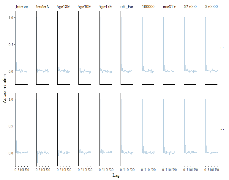
Autocorrelation check. In our chase we can assume that there is no problem with autocorrelation because the autocorr parameters quickly drop to around zero.
stanplot(Bayes_Model_SW,
         type = "acf_bar")
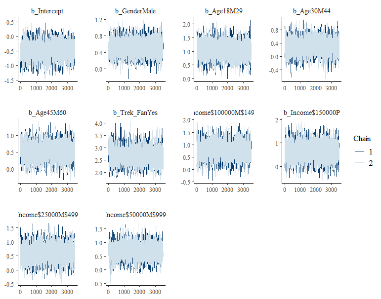
Chain convergence check. No indication of convergence problems since the chains mix well for all variables.
stanplot(Bayes_Model_SW,
         type = "trace")
Summary Bayesian Logit model
Since there was no indication that our modeling did not work out as expected, we can now continue to look at our results.
summary(Bayes_Model_SW)
##  Family: bernoulli
##   Links: mu = logit
## Formula: Watched_SW ~ Gender + Age + Trek_Fan + Income
##    Data: starwars_data (Number of observations: 858)
##   Draws: 2 chains, each with iter = 4000; warmup = 500; thin = 1;
##          total post-warmup draws = 7000
##
## Population-Level Effects:
##                       Estimate Est.Error l-95% CI u-95% CI Rhat
## Intercept                -0.49      0.28    -1.04     0.05 1.00
## GenderMale                0.53      0.19     0.16     0.90 1.00
## Age18M29                  1.05      0.29     0.50     1.62 1.00
## Age30M44                  0.30      0.23    -0.15     0.76 1.00
## Age45M60                  0.52      0.25     0.04     1.01 1.00
## Trek_FanYes               2.68      0.32     2.09     3.35 1.00
## Income$100000M$149999     0.77      0.32     0.14     1.43 1.00
## Income$150000P            0.63      0.36    -0.07     1.36 1.00
## Income$25000M$49999       0.61      0.29     0.04     1.18 1.00
## Income$50000M$99999       0.69      0.27     0.16     1.23 1.00

##
## Draws were sampled using sampling(NUTS). For each parameter, Bulk_ESS
## and Tail_ESS are effective sample size measures, and Rhat is the potential
## scale reduction factor on split chains (at convergence, Rhat = 1).
If we compare the Estimates of the normal/Frequentist Logit model and the Bayesian Logit model we see that the estimates are quite similar. But instead of significance values, the Bayesian Logit model shows Credibility Intervals for the effects. The go adrift from rigid (relative arbitrary) significance cut-offs (is there really such a big difference between 0.06 and 0.049???) and the turning to CrI is in my opinion a big advantage of this approach.
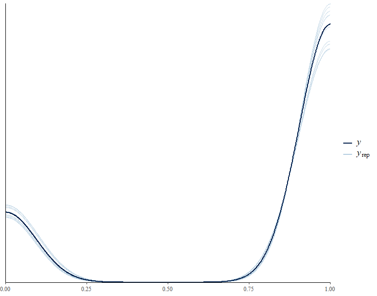
Posterior prediction check
Posterior predictive check lets us inspect what the model suggests for our Y variable (watched at least one StarWars movie) vs. what actually is the case.
From our posterior prediction plot we see that our model is fitting the observed Star Wars data quite well.
pp_check(Bayes_Model_SW)
## Using 10 posterior draws for ppc type 'dens_overlay' by default.
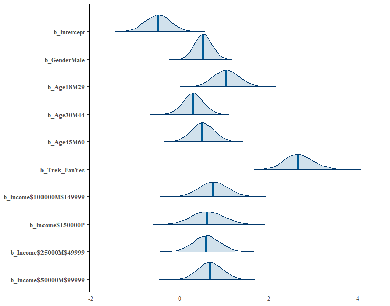
Visualize effect ranges
The plot show the visual effect credibility interval (CrI). With a likelihood of 97.5% the effect of StarTrek ranges from 2.09-3.35 (mean 2.68).
But note that these ranges still represent log odds. If you want to interpret them be careful. A statement like the following would be ok though: Being a StarTrek Fan is associated with a 2.68 increase in log odds of having at least watched one Star Wars movie.
stanplot(Bayes_Model_SW,
         type = "areas",
         prob = 0.975)