Linear regression with NFL data
We want to check if different characteristics like passing and rush yards predict the score of the possessing team. In order to check this (and other relationships) we will use a real-word dataset containing 407688 observations and 102 variables about real NFL plays from 2009 to 2017.
The dataset (V4) can be found under: https://www.kaggle.com/datasets/maxhorowitz/nflplaybyplay2009to2016?select=NFL+Play+by+Play+2009-2017+%28v4%29.csv
Required libraries
library(stats)
library(dplyr)
library(ggplot2)
library(car)
Load the dataset
NFL_data_all <- read.csv("your_path", sep = ",")
Data preparation
We first select the columns we want to work with, rename and make sure they have the right class (numeric, factors). We choose Score possessing team as a dependent variable and all the others as independent variables (also called predictors)
#select needed columns for analyses
NFL_selected_var <- as.data.frame(cbind(NFL_data_all$GameID, NFL_data_all$posteam, NFL_data_all$ï..Date,   NFL_data_all$PosTeamScore, NFL_data_all$PlayType, NFL_data_all$Yards.Gained, NFL_data_all$Fumble, NFL_data_all$InterceptionThrown, NFL_data_all$RushAttempt, NFL_data_all$PassAttempt, NFL_data_all$Sack))

# rename columns
colnames(NFL_selected_var) <- c("Game_id", "Possessing_team", "Game_date", "Score_poss_team", "Play_type", "Yards_gained", "Fumble", "Interception", "Rush_attempts", "Pass_attempts", "Sack")

cols_factors <- c("Play_type")
cols_numeric <- c("Score_poss_team", "Yards_gained", "Rush_attempts", "Pass_attempts", "Fumble", "Interception", "Sack")

NFL_selected_var[cols_factors] <- lapply(NFL_selected_var[cols_factors], factor) # convert column values to factor levels
NFL_selected_var[cols_numeric] <- lapply(NFL_selected_var[cols_numeric], as.numeric) # convert column values to numeric
Afterwards we are calculate a new three new variables: season, rush yards, passing yards
# create season variable from game_date
# There is also a Season variable but i wanted to show how to extract years from data
NFL_selected_var$Season <- format(as.Date(NFL_selected_var$Game_date, format="%Y-%m-%d"),"%Y")

# if variable Pass_attempts is 1, we want the number of Yards_gained stored in our new variable Passing_yards
NFL_selected_var <-NFL_selected_var %>%
  mutate(Passing_yards = ifelse(Pass_attempts == 1, Yards_gained, 0))

NFL_selected_var <-NFL_selected_var %>%
  mutate(Rushing_yards = ifelse(Rush_attempts == 1, Yards_gained, 0))
Remove missing values and create some more interesting variables
# Since we are just interested in the plays that are correctly specified (pass, run, sack), we can use those factor levels to subset our data and just ignore all plays that are misspecified with NA

NFL_selected_var_clean <- filter(NFL_selected_var, Play_type %in% c("Pass", "Run", "Sack")) %>%
  group_by(Game_id, Possessing_team, Season) #only 290833 observations left

# We can check the play by play data (not all columns are shown)
head(NFL_selected_var_clean)
## # A tibble: 6 x 14
## # Groups:   Game_id, Possessing_team, Season [2]
##   Game_id    Possessing_team Game_date  Score_poss_team Play_type Yards_gained
##   <chr>      <chr>           <chr>                <dbl> <fct>            <dbl>
## 1 2009091000 PIT             2009-09-10               0 Pass                 5
## 2 2009091000 PIT             2009-09-10               0 Run                 -3
## 3 2009091000 PIT             2009-09-10               0 Pass                 0
## 4 2009091000 TEN             2009-09-10               0 Run                  0
## 5 2009091000 TEN             2009-09-10               0 Pass                 4
## 6 2009091000 TEN             2009-09-10               0 Run                 -2
## # ... with 8 more variables: Fumble <dbl>, Interception <dbl>,
## #   Rush_attempts <dbl>, Pass_attempts <dbl>, Sack <dbl>, Season <chr>,
## #   Passing_yards <dbl>, Rushing_yards <dbl>
Summerize (condense) dataset further and describe it
# Since we are just interested in the plays that are correctly specified (pass, run, sack), we can use those factor levels to subset our data and just ignore all plays that are misspecified with NA

Stats_per_Team_Season <- NFL_selected_var_clean %>%
  summarize(Score=max(Score_poss_team),
  PassYards = sum(Passing_yards),
  RushYards = sum(Rushing_yards),
  TotalYards = sum(Passing_yards+Rushing_yards),
  RushAttempts = sum(Rush_attempts),
  PassAttempts = sum(Pass_attempts),
  Fumbles = sum(Fumble),
  Sacks = sum(Sack),
  Interceptions = sum(Interception),
  PassPerc = PassAttempts/(RushAttempts+PassAttempts), # percentage of pass game in relation to the running game
  AvgRush = (RushYards/RushAttempts), # average rushing yards
  AvgPass = (PassYards/PassAttempts)) %>% # average passing yards
  filter(Possessing_team != "")
# check our new dataframe - it shows the averages for specific team for a specific game (see Game_id)
head(Stats_per_Team_Season)
## # A tibble: 6 x 15
## # Groups:   Game_id, Possessing_team [6]
##   Game_id    Possessing_team Season Score PassYards RushYards TotalYards
##   <chr>      <chr>           <chr>  <dbl>     <dbl>     <dbl>      <dbl>
## 1 2009091000 PIT             2009      10       363        36        399
## 2 2009091000 TEN             2009      10       244        86        330
## 3 2009091300 ATL             2009      19       229        72        301
## 4 2009091300 MIA             2009       0       182        96        278
## 5 2009091301 BAL             2009      31       312       198        510
## 6 2009091301 KC              2009      23       177        29        206
## # ... with 8 more variables: RushAttempts <dbl>, PassAttempts <dbl>,
## #   Fumbles <dbl>, Sacks <dbl>, Interceptions <dbl>, PassPerc <dbl>,
## #   AvgRush <dbl>, AvgPass <dbl>
# average across all teams (season 2009-2017)
summary(Stats_per_Team_Season[4:15])
##      Score        PassYards     RushYards       TotalYards     RushAttempts
##  Min.   : 0.0   Min.   :  0   Min.   :  1.0   Min.   : 87.0   Min.   : 7.00
##  1st Qu.:14.0   1st Qu.:194   1st Qu.: 78.0   1st Qu.:306.0   1st Qu.:21.00
##  Median :20.0   Median :244   Median :108.0   Median :362.0   Median :26.00
##  Mean   :20.7   Mean   :248   Mean   :114.5   Mean   :362.5   Mean   :26.21
##  3rd Qu.:27.0   3rd Qu.:299   3rd Qu.:145.0   3rd Qu.:418.0   3rd Qu.:31.00
##  Max.   :61.0   Max.   :675   Max.   :363.0   Max.   :792.0   Max.   :60.00
##   PassAttempts      Fumbles          Sacks        Interceptions
##  Min.   : 7.00   Min.   :0.000   Min.   : 0.000   Min.   :0.0000
##  1st Qu.:29.00   1st Qu.:0.000   1st Qu.: 1.000   1st Qu.:0.0000
##  Median :34.00   Median :1.000   Median : 2.000   Median :1.0000
##  Mean   :34.61   Mean   :1.116   Mean   : 2.311   Mean   :0.9362
##  3rd Qu.:40.00   3rd Qu.:2.000   3rd Qu.: 3.000   3rd Qu.:1.0000
##  Max.   :70.00   Max.   :9.000   Max.   :11.000   Max.   :6.0000
##     PassPerc         AvgRush          AvgPass
##  Min.   :0.1290   Min.   : 0.100   Min.   : 0.000
##  1st Qu.:0.4930   1st Qu.: 3.385   1st Qu.: 5.941
##  Median :0.5714   Median : 4.173   Median : 7.094
##  Mean   :0.5683   Mean   : 4.292   Mean   : 7.249
##  3rd Qu.:0.6464   3rd Qu.: 5.059   3rd Qu.: 8.341
##  Max.   :0.8727   Max.   :13.562   Max.   :16.133
We can see that on average 20.7 points were scored in teh NFL from 2009-2017. Passing yards on average were 248.0 while rushing yards on average were 114.5. Note that the max total yards include an unrealistic outlier (max 792.0). Average rush yards were 4.29 and average passing yards were 7.25. Nearly one interception, 2.3 sacks and slightly more than one fumble was produced by the teams. Further we can see that on average ~ 57% were passing plays (var. PassPerc).
Dealing with outliers
Since we saw the max 792.0 yards in one game cant be right (according to a Google search: LA Rams is the record holder with 722 yards in 1951 against the New York Yanks), we can deal with outliers (or wrongly captured values in our dataset)
Stats_per_Team_Season <- Stats_per_Team_Season[!is.na(Stats_per_Team_Season$TotalYards), ]
Q <- quantile(Stats_per_Team_Season$TotalYards, probs=c(.25, .75), na.rm = FALSE) # set 25/75% quantile
iqr <- IQR(Stats_per_Team_Season$TotalYards)

Stats_per_Team_Season_wOL<- subset(Stats_per_Team_Season, Stats_per_Team_Season$TotalYards > (Q[1] - 1.5*iqr) & Stats_per_Team_Season$TotalYards < (Q[2]+1.5*iqr))
Simple linear regression analysis
A simple regression analysis includes one independent variable (often called X variable) and one dependent variable (often called Y variable). We want to check if in increase of X also significantly increases Y. In our case we assume that the amount of total yards a team makes also increases the teams score (total yards –> teams score)
Before we calculate our simple regression model, we have to check if the relation between our two variables is actually linear. I will check it visually via scatterplot. (I recommend to have a look at your data everytime you want to analyze something)
# We use our summerized dataset
scatterplot(Score ~ TotalYards, data = Stats_per_Team_Season_wOL, frame = FALSE)
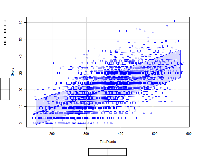
We see that there is still quite a high variation (some teams with little yards and a lot of points - the plot also identifies those as outliers which is shown in the boxplot on the y-axis) but still a general linear trend is visible.
# Now we build our simple linear regression model with X = TotalYards and Y = Score
set.seed(42)

simple_regression_model <- lm(Score ~ TotalYards, data=Stats_per_Team_Season_wOL)
summary(simple_regression_model)
##
## Call:
## lm(formula = Score ~ TotalYards, data = Stats_per_Team_Season_wOL)
##
## Residuals:
##     Min      1Q  Median      3Q     Max
## -23.568  -5.477  -0.444   4.789  31.882
##
## Coefficients:
##             Estimate Std. Error t value Pr(>|t|)
## (Intercept) -4.71246    0.53690  -8.777   <2e-16 ***
## TotalYards   0.07010    0.00145  48.331   <2e-16 ***
## ---
## Signif. codes:  0 '***' 0.001 '**' 0.01 '*' 0.05 '.' 0.1 ' ' 1
##
## Residual standard error: 7.859 on 4571 degrees of freedom
## Multiple R-squared:  0.3382, Adjusted R-squared:  0.3381
## F-statistic:  2336 on 1 and 4571 DF,  p-value: < 2.2e-16
Next we interpret the reuslts of our simple linear regression model. We start with the overall fit indicated by the F-statistic. Here we can see that the overall model is significant (p < 0.05). The explained variance (indicated by the multiple R-squared) is ok with 0.3382. Afterwards we can interpret our coefficient. For our used dataset we see the independent variable TotalYards does significantly increase our dependent variable Score (ß = 0.070, p < 0.01). Meaning, when we increase TotalYars by one unit, Score will increase by 0.07.
Multiple linear regression analysis
In the simple regression we saw that TotalYards have an sigificant effect on Score. But the predicitive power of our simple model was rather mediocre (indicated by a low R-squared). This suggests that we have not taken all relevant variables into account in our simple regression model. Therefore we now want to calculate a multiple linear regression model. A multiple linear regression model includes MULTIPLE independent variables (2 or more X variables) and one dependent variable.
In our case we want to check if the independent variables PassYards, RushYards, PassAttempts, RushAttempts, Interceptions, Fumbles and Sacks in the game do predict Score better than our simple linear regression model.
# Now we build our multiple linear regression model with X = several independent variables and Y = Score
set.seed(42)

mulitple_regression_model <- lm(Score ~ PassYards + RushYards + PassAttempts + RushAttempts + Interceptions + Fumbles + Sacks, data=Stats_per_Team_Season_wOL)

summary(mulitple_regression_model)
##
## Call:
## lm(formula = Score ~ PassYards + RushYards + PassAttempts + RushAttempts +
##     Interceptions + Fumbles + Sacks, data = Stats_per_Team_Season_wOL)
##
## Residuals:
##      Min       1Q   Median       3Q      Max
## -23.0255  -4.7152  -0.4153   4.3563  26.5850
##
## Coefficients:
##                Estimate Std. Error t value Pr(>|t|)
## (Intercept)    6.477701   0.781209   8.292  < 2e-16 ***
## PassYards      0.078731   0.001784  44.123  < 2e-16 ***
## RushYards      0.053846   0.003046  17.677  < 2e-16 ***
## PassAttempts  -0.311628   0.017593 -17.713  < 2e-16 ***
## RushAttempts   0.134036   0.021818   6.143 8.77e-10 ***
## Interceptions -1.395667   0.106014 -13.165  < 2e-16 ***
## Fumbles       -0.679940   0.094075  -7.228 5.73e-13 ***
## Sacks         -0.923205   0.062574 -14.754  < 2e-16 ***
## ---
## Signif. codes:  0 '***' 0.001 '**' 0.01 '*' 0.05 '.' 0.1 ' ' 1
##
## Residual standard error: 6.823 on 4565 degrees of freedom
## Multiple R-squared:  0.5018, Adjusted R-squared:  0.5011
## F-statistic: 656.9 on 7 and 4565 DF,  p-value: < 2.2e-16
Again the F-statisitcs is significant indicating that at least one of our X variaibles has a significant effect. The R-squared increased from ~ 33% to over 50%. And our coefficients all have a significant impact on Score. PassYards, RushYards, RushAttempts do have a positive effect on Score, while Interceptions, Fumbles and Sacks have a negative effect on Score (because defense wins championships!). Surprisingly, PassAttempts also have a negative effect. A possible explanation could be that passing game is more prone to interceptions and incomplete passes (0 yards), especially when teams are under pressure to score. In a last step we want to check how the negative effect looks like by plotting a scatterplot.
# Now we build our multiple linear regression model with X = several independent variables and Y = Score
set.seed(42)

scatterplot(Score~PassAttempts, data = Stats_per_Team_Season_wOL, frame=FALSE)
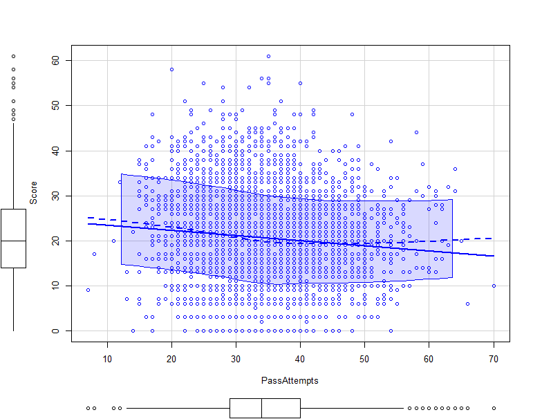
Note: The data distribution is quite focused on the middle and there seems to be little correlation between Score and PassAttempts. Therefore, interpret with caution.