Pandemic netflix consumption
During the pandemic 2020-2022 in the US
In this post I would like to look at some netflix data containing daily TOP10 on Netflix US during pandemic (04/2020-04/2022). Specifically, the dataset includes variables like Title (of the show/movie), the daily rank, the summed up count for being in the TOP10, the type (tv show/movie) and the viewership score.
The data source is https://www.the-numbers.com/netflix-top-10
Note: Use at your own risk. Be ethical about (user) data. This post will showcase how you can use simple statistics on everyday phenomena.
Required libraries
library(dplyr)
library(ggplot2)
library(stringr)
library(rstatix)
Looking at the data
After loading the data set, we look at the data (first 5 rows)
head(netflix_binge_data, 5)
##         As.of Rank Year.to.Date.Rank Last.Week.Rank  Title          Type       Netflix.Exclusive  Netflix.Release.Date   Days.In.Top.10   Viewership.Score
## 1  2020-04-01    1                 1              1  Tiger King     TV Show                  Yes          Mar 20, 2020                9                 90
## 2  2020-04-01    2                 2              -  Ozark          TV Show                  Yes          Jul 21, 2017                5                 45
## 3  2020-04-01    3                 3              2  All American   TV Show                               Mar 28, 2019                9                 76
## 4  2020-04-01    4                 4              -  Blood Father   Movie                                 Mar 26, 2020                5                 30
## 5  2020-04-01    5                 5              4  The Platform   Movie                    Yes          Mar 20, 2020                9                 55
Some overall descriptives
Check if TV shows or movies dominated the TOP 10 in pandemic times.
netflix_binge_data %>% dplyr::count(Type, sort = TRUE)
##              Type    n
## 1         TV Show 4446
## 2           Movie 2611
## 3 Stand-Up Comedy   41
## 4   Concert/Perf…    2
TV shows do dominate the daily Top 10. Since this is time-series data, a show is counted multiple times. On day to day basis TV shows (n = 4446) are more frequently in the daily TOP 10 than Movie (n = 2611). This difference might be explained by the fact that watching a TV show with episodes takes longer or that the pandemic time increased binge watching habits.
Next we check what shows stayed in the TOP 10 the longest.
Days_in_top10 <- netflix_binge_data %>% dplyr::count(Title, sort = TRUE)

# Take a look at the TOP20 of the TOP10

head(Days_in_top10, 20)
##                                 Title   n
## 1                           Cocomelon 428
## 2                               Ozark  85
## 3                           Cobra Kai  81
## 4                            Manifest  80
## 5                  The Queen's Gambit  73
## 6                         Outer Banks  72
## 7                          Squid Game  66
## 8                        All American  58
## 9                          Bridgerton  58
## 10                            Lucifer  56
## 11                       Virgin River  55
## 12                               Maid  49
## 13                     Emily in Paris  48
## 14                  Too Hot to Handle  47
## 15                    Sweet Magnolias  45
## 16                        The Witcher  45
## 17                    Ginny & Georgia  44
## 18                  The Queen of Flow  44
## 19                             iCarly  42
## 20                          Shameless  42
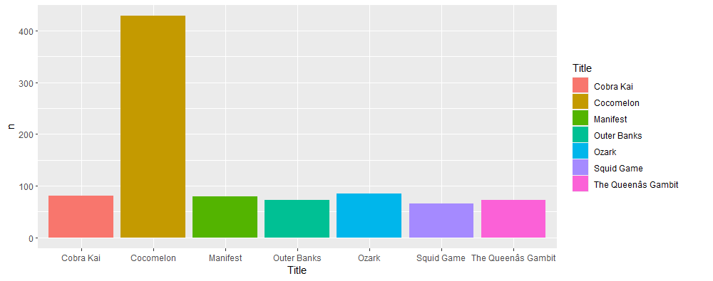
Interestingly or alarmingly, Cocomelon a TV show (audiance: preschool kids) is the TV show longest in the daily TOP 10 in the US over the course of the pandemic time 2020-2022 with 428 days. Followed by Ozak (85 days). Other shows like Cobra Kai (81 days), Squid Game (66 days) are behind by far. Movies are rarely longer than 15 days in the TOP 10.

Visualization
First filter (excluding all movie/series mentioned less than 60 times) and using ggplot to visualize
Days_in_top10 %>%
  filter(n >= 60) %>%
  ggplot(Days_in_top10, mapping =  aes(Title, n, fill=Title))+ geom_bar(stat='identity')
Analyze your own TV shows/movies/Create own subset of data
Use str_detect (stringr package) to filter for specific shows and factorize the show titles.
Show_comparison_pandemic <- netflix_binge_data %>%
  filter(str_detect(netflix_binge_data[,5], 'Squid Game|Ozark|Bridgerton|Tiger King: Murder|Money Heist|Cobra Kai'))

# factorize the show title
Show_comparison_pandemic$Title <- as.factor(Show_comparison_pandemic$Title)
Calculate mean rank
Using aggregate function to calculate the mean rank for the chosen shows plus we use ggplot 2 to visualize these means
aggregate(Show_comparison_pandemic$Rank ~ Show_comparison_pandemic$Title, FUN = mean)
##   Show_comparison_pandemic$Title Show_comparison_pandemic$Rank
## 1                     Bridgerton                      3.551724
## 2                      Cobra Kai                      3.814815
## 3                    Money Heist                      4.846154
## 4                          Ozark                      5.117647
## 5                     Squid Game                      3.500000
## 6   Tiger King: Murder, Mayhem …                      2.724138
We see that tiger King has the best average ranking with m = 2.72, followed by Squid Game (m = 3.50) and Bridgerton (m = 3.55). From the selected shows Ozark (m = 5.12) has the worst average ranking.
ggplot(Show_comparison_pandemic, aes(x = factor(Title), y = Rank, fill=Title)) +
  geom_bar(stat = "summary", fun = "mean")
![]()
Multiple mean comparison
After the visualization shows obvious differences, we use a multiple mean comparison (from rstatix package) to check if the differences are rather significant or random.
Show_comparison_pandemic %>%
  t_test(Rank ~ Title) %>%
  adjust_pvalue(method = "BH")%>%
  add_significance()
## # A tibble: 15 x 10
##    .y.   group1  group2    n1    n2 statistic    df       p   p.adj p.adj.signif
##  * <chr> <chr>   <chr>  <int> <int>     <dbl> <dbl>   <dbl>   <dbl> <chr>
##  1 Rank  Bridge~ Cobra~    58    81   -0.522  123.  6.02e-1 0.677   ns
##  2 Rank  Bridge~ Money~    58    39   -2.13    81.4 3.6 e-2 0.0771  ns
##  3 Rank  Bridge~ Ozark     58    85   -3.17   121.  2   e-3 0.01    **
##  4 Rank  Bridge~ Squid~    58    66    0.0968 121.  9.23e-1 0.923   ns
##  5 Rank  Bridge~ Tiger~    58    29    1.32    61.2 1.91e-1 0.286   ns
##  6 Rank  Cobra ~ Money~    81    39   -1.80    74.8 7.6 e-2 0.127   ns
##  7 Rank  Cobra ~ Ozark     81    85   -2.89   163.  4   e-3 0.012   *
##  8 Rank  Cobra ~ Squid~    81    66    0.638  137.  5.25e-1 0.656   ns
##  9 Rank  Cobra ~ Tiger~    81    29    1.84    54.1 7   e-2 0.127   ns
## 10 Rank  Money ~ Ozark     39    85   -0.481   72.1 6.32e-1 0.677   ns
## 11 Rank  Money ~ Squid~    39    66    2.24    81.4 2.8 e-2 0.07    ns
## 12 Rank  Money ~ Tiger~    39    29    3.11    63.5 3   e-3 0.0112  *
## 13 Rank  Ozark   Squid~    85    66    3.34   136.  1   e-3 0.0075  **
## 14 Rank  Ozark   Tiger~    85    29    4.10    51.9 1.44e-4 0.00216 **
## 15 Rank  Squid ~ Tiger~    66    29    1.26    60.3 2.14e-1 0.292   ns
The test shows us that the rank of Bridgerton & Ozark, Cobra Kai & Ozark, Money Heist & Tiger King, Ozark & Squid Game and Ozark & Tiger King differ significantly. (Should be interpreted with caution, as the distribution of data points (n1/n2) is quite uneven)