RScript from R Introduction Workshop
This is a script from my latest R Introduction Workshop
Modified data from ‘https://towardsdatascience.com/structural-equation-modeling-dca298798f4d’ was used. Thanks to the author to upload the dataset in a data s3 bucket. If you want to replicate this Workshop, check the data prep code in this post!
Required libraries
library(ggplot2)
library(dplyr)
library(car)
library(outliers)
library(stats)
library(rstatix)
library(ggpubr)
library(QuantPsyc)
library(psych)
library(lavaan)
library(semPlot)
library(semTools)
The data was renamed and a product variable was added to make it more suitable for the courses context.
Data prep
BR_data <- read.csv('https://articledatas3.s3.eu-central-1.amazonaws.com/StructuralEquationModelingData.csv')

names(BR_data)[names(BR_data) == "PsychTest1"] <- "TV_spent"
names(BR_data)[names(BR_data) == "PsychTest2"] <- "SoMed_spent"
names(BR_data)[names(BR_data) == "YrsEdu"] <- "Custom_rating"
names(BR_data)[names(BR_data) == "IQ"] <- "Test_rating"
names(BR_data)[names(BR_data) == "HrsTrn"] <- "Dura_score"
names(BR_data)[names(BR_data) == "HrsWrk"] <- "Function_score"

names(BR_data)[names(BR_data) == "ClientSat"] <- "Sales"
names(BR_data)[names(BR_data) == "SuperSat"] <- "Brand_trust"
names(BR_data)[names(BR_data) == "ProjCompl"] <- "Emotion_appeal"

BR_data$Product <- with(BR_data, ifelse(Sales > 70, 'A',
                              ifelse(Sales > 45 , 'B', 'C')))
First visual approach & missing values
# look at data set (first 5 rows)
head(BR_data, 5)
##   TV_spent SoMed_spent Custom_rating Test_rating Dura_score Function_score
## 1       62          78             5          97          6             33
## 2       46          27             2          93          7             54
## 3       68          75             2          96          5             47
## 4       55          56             4         103          7             80
## 5       51          32             4          98          5             53
##   Sales Brand_trust Emotion_appeal Product
## 1    84          59             34       A
## 2    55          38             56       B
## 3    70          68             38       B
## 4    63          81             78       B
## 5    55          39             56       B
View(BR_data) # show entire data set in new tab

# check for missing value in a variable
table(BR_data$TV_spent, exclude = NULL)
##
## 20 21 22 24 25 26 27 28 29 30 31 32 33 34 35 36 37 38 39 40 41 42 43 44 45 46
##  2  2  1  3  3  4  3  1  2  4  9  7 15 11 13  8 21 26 15 23 22 25 34 27 37 46
## 47 48 49 50 51 52 53 54 55 56 57 58 59 60 61 62 63 64 65 66 67 68 69 70 71 72
## 34 39 46 33 37 41 40 33 31 33 35 37 31 25 19 18 20 10  9 16  5  8  9  7  9  4
## 73 74 75 78 81
##  1  3  1  1  1
# count of missing values
sum(is.na(BR_data))
## [1] 0
# finds the location of missing values
which(is.na(BR_data))
## integer(0)
# finds missing values in columns
sapply(BR_data, function(x) sum(is.na(x)))
##       TV_spent    SoMed_spent  Custom_rating    Test_rating     Dura_score
##              0              0              0              0              0
## Function_score          Sales    Brand_trust Emotion_appeal        Product
##              0              0              0              0              0
# replace missing values with zeros
BR_data[is.na(BR_data)] <- 0
Descriptives
str(BR_data) # structure of data set
## 'data.frame':    1000 obs. of  10 variables:
##  $ TV_spent      : int  62 46 68 55 51 51 55 55 50 55 ...
##  $ SoMed_spent   : int  78 27 75 56 32 66 40 64 33 36 ...
##  $ Custom_rating : int  5 2 2 4 4 3 0 1 2 0 ...
##  $ Test_rating   : int  97 93 96 103 98 102 98 95 96 94 ...
##  $ Dura_score    : int  6 7 5 7 5 10 8 7 10 6 ...
##  $ Function_score: int  33 54 47 80 53 56 54 75 69 68 ...
##  $ Sales         : int  84 55 70 63 55 63 61 58 63 66 ...
##  $ Brand_trust   : int  59 38 68 81 39 68 53 71 61 56 ...
##  $ Emotion_appeal: int  34 56 38 78 56 57 53 75 62 63 ...
##  $ Product       : chr  "A" "B" "B" "B" ...
# convert to factor
BR_data$Product <- as.factor(BR_data$Product)

# summarize descriptive stats
summary(BR_data)
##     TV_spent      SoMed_spent    Custom_rating    Test_rating
##  Min.   :20.00   Min.   : 5.00   Min.   :0.000   Min.   : 90.00
##  1st Qu.:43.00   1st Qu.:38.75   1st Qu.:1.000   1st Qu.: 95.00
##  Median :50.00   Median :50.00   Median :3.000   Median : 97.00
##  Mean   :49.99   Mean   :49.29   Mean   :2.506   Mean   : 97.59
##  3rd Qu.:57.00   3rd Qu.:60.00   3rd Qu.:4.000   3rd Qu.:101.00
##  Max.   :81.00   Max.   :90.00   Max.   :5.000   Max.   :105.00
##    Dura_score     Function_score       Sales         Brand_trust
##  Min.   : 0.000   Min.   :  0.00   Min.   :  0.00   Min.   :  0.00
##  1st Qu.: 4.000   1st Qu.: 30.00   1st Qu.: 43.00   1st Qu.: 38.00
##  Median : 6.000   Median : 47.00   Median : 55.00   Median : 50.00
##  Mean   : 6.028   Mean   : 47.81   Mean   : 54.97   Mean   : 49.91
##  3rd Qu.: 8.000   3rd Qu.: 64.00   3rd Qu.: 67.00   3rd Qu.: 62.00
##  Max.   :17.000   Max.   :100.00   Max.   :100.00   Max.   :100.00
##  Emotion_appeal   Product
##  Min.   :  0.00   A:186
##  1st Qu.: 33.00   B:515
##  Median : 48.00   C:299
##  Mean   : 48.13
##  3rd Qu.: 63.00
##  Max.   :100.00
# if you need stats by a column
by(BR_data, BR_data$Product, summary)
## BR_data$Product: A
##     TV_spent      SoMed_spent    Custom_rating    Test_rating
##  Min.   :46.00   Min.   :27.00   Min.   :0.000   Min.   : 90.00
##  1st Qu.:58.00   1st Qu.:52.00   1st Qu.:2.000   1st Qu.: 95.00
##  Median :62.00   Median :61.00   Median :3.000   Median : 98.00
##  Mean   :62.53   Mean   :60.72   Mean   :2.973   Mean   : 97.99
##  3rd Qu.:67.00   3rd Qu.:71.00   3rd Qu.:4.000   3rd Qu.:101.00
##  Max.   :81.00   Max.   :90.00   Max.   :5.000   Max.   :105.00
##    Dura_score     Function_score       Sales         Brand_trust
##  Min.   : 1.000   Min.   :  0.00   Min.   : 71.00   Min.   : 17.0
##  1st Qu.: 4.250   1st Qu.: 31.25   1st Qu.: 75.00   1st Qu.: 47.0
##  Median : 6.000   Median : 49.50   Median : 80.00   Median : 61.0
##  Mean   : 6.478   Mean   : 50.97   Mean   : 81.15   Mean   : 59.1
##  3rd Qu.: 8.000   3rd Qu.: 69.75   3rd Qu.: 87.00   3rd Qu.: 71.0
##  Max.   :14.000   Max.   :100.00   Max.   :100.00   Max.   :100.0
##  Emotion_appeal  Product
##  Min.   : 4.00   A:186
##  1st Qu.:34.00   B:  0
##  Median :52.50   C:  0
##  Mean   :51.08
##  3rd Qu.:68.00
##  Max.   :96.00
## ------------------------------------------------------------
## BR_data$Product: B
##     TV_spent      SoMed_spent    Custom_rating    Test_rating
##  Min.   :33.00   Min.   :16.00   Min.   :0.000   Min.   : 90.00
##  1st Qu.:47.00   1st Qu.:41.00   1st Qu.:1.000   1st Qu.: 95.00
##  Median :51.00   Median :50.00   Median :3.000   Median : 97.00
##  Mean   :51.45   Mean   :50.73   Mean   :2.544   Mean   : 97.59
##  3rd Qu.:56.00   3rd Qu.:60.00   3rd Qu.:4.000   3rd Qu.:101.00
##  Max.   :68.00   Max.   :83.00   Max.   :5.000   Max.   :105.00
##    Dura_score     Function_score      Sales        Brand_trust
##  Min.   : 0.000   Min.   :  0.0   Min.   :46.00   Min.   : 0.00
##  1st Qu.: 4.000   1st Qu.: 29.5   1st Qu.:52.00   1st Qu.:40.00
##  Median : 6.000   Median : 48.0   Median :57.00   Median :52.00
##  Mean   : 6.146   Mean   : 48.3   Mean   :57.65   Mean   :51.09
##  3rd Qu.: 8.000   3rd Qu.: 65.0   3rd Qu.:64.00   3rd Qu.:63.00
##  Max.   :17.000   Max.   :100.0   Max.   :70.00   Max.   :95.00
##  Emotion_appeal   Product
##  Min.   :  2.00   A:  0
##  1st Qu.: 33.00   B:515
##  Median : 48.00   C:  0
##  Mean   : 48.68
##  3rd Qu.: 64.00
##  Max.   :100.00
## ------------------------------------------------------------
## BR_data$Product: C
##     TV_spent      SoMed_spent    Custom_rating    Test_rating
##  Min.   :20.00   Min.   : 5.00   Min.   :0.000   Min.   : 90.00
##  1st Qu.:35.00   1st Qu.:31.00   1st Qu.:1.000   1st Qu.: 94.00
##  Median :40.00   Median :39.00   Median :2.000   Median : 97.00
##  Mean   :39.67   Mean   :39.68   Mean   :2.151   Mean   : 97.32
##  3rd Qu.:45.00   3rd Qu.:50.50   3rd Qu.:4.000   3rd Qu.:101.00
##  Max.   :58.00   Max.   :69.00   Max.   :5.000   Max.   :105.00
##    Dura_score     Function_score     Sales        Brand_trust
##  Min.   : 1.000   Min.   :  0    Min.   : 0.00   Min.   : 2.00
##  1st Qu.: 4.000   1st Qu.: 30    1st Qu.:29.50   1st Qu.:30.50
##  Median : 5.000   Median : 45    Median :36.00   Median :43.00
##  Mean   : 5.545   Mean   : 45    Mean   :34.07   Mean   :42.17
##  3rd Qu.: 7.000   3rd Qu.: 59    3rd Qu.:41.00   3rd Qu.:52.00
##  Max.   :14.000   Max.   :100    Max.   :45.00   Max.   :87.00
##  Emotion_appeal  Product
##  Min.   : 0.00   A:  0
##  1st Qu.:32.00   B:  0
##  Median :45.00   C:299
##  Mean   :45.35
##  3rd Qu.:58.00
##  Max.   :96.00
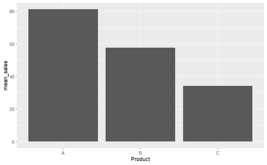
# let plot mean of Sales
# first create data frame with means of Sales
# create a new dataframe crop_means
Sales_means <- BR_data %>%
  group_by(Product) %>%
  summarize(mean_sales=mean(Sales))
Sales_means
## # A tibble: 3 x 2
##   Product mean_sales
##   <fct>        <dbl>
## 1 A             81.2
## 2 B             57.6
## 3 C             34.1
#second - plotting using ggplot
ggplot(Sales_means, aes(x=Product, y=mean_sales)) +
  geom_bar(stat="identity")
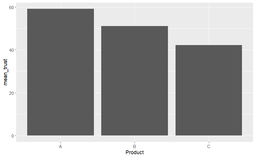
# another example looking at brand trust
Trust_means <- BR_data %>%
  group_by(Product) %>%
  summarize(mean_trust=mean(Brand_trust))
Trust_means
## # A tibble: 3 x 2
##   Product mean_trust
##   <fct>        <dbl>
## 1 A             59.1
## 2 B             51.1
## 3 C             42.2
ggplot(Trust_means, aes(x=Product, y=mean_trust)) +
  geom_bar(stat="identity")
ANOVA
##### ANOVA #####
# now lets check if sales between product is significantly different
# compute ANOVA
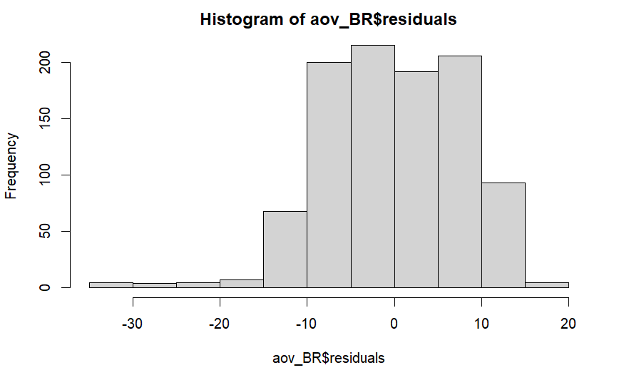
aov_BR <- aov(Sales ~ Product, data = BR_data)
# 1st: test normality of the residuals with the Shapiro-Wilk test
shapiro.test(aov_BR$residuals) # p-value of the Shapiro-Wilk test is significant --> normality assumption violated
##
##  Shapiro-Wilk normality test
##
## data:  aov_BR$residuals
## W = 0.96461, p-value = 7.318e-15
hist(aov_BR$residuals) # visual conformation of ignore this test
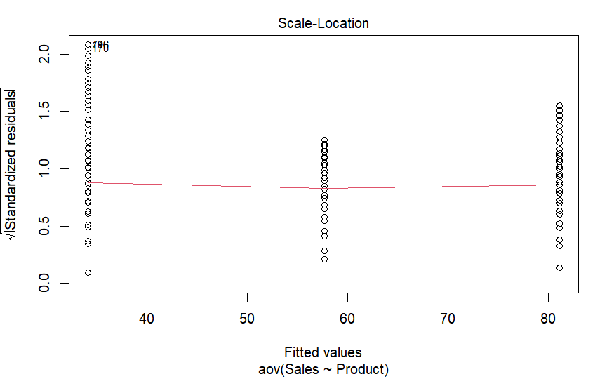
# 2nd: test for homogeneity of variances with Levene-Test
leveneTest(Sales ~ Product, data = BR_data)# p-value indicates violation of assumption of homogeneity of variances
## Levene's Test for Homogeneity of Variance (center = median)
##        Df F value   Pr(>F)
## group   2  6.6952 0.001293 **
##       997
## ---
## Signif. codes:  0 '***' 0.001 '**' 0.01 '*' 0.05 '.' 0.1 ' ' 1
plot(aov_BR, which = 3) # visual inspection show a more indeifferent pciture. Line is not entirely straight - more likely a violation of assumption of homogeneity of variances. But for the sake of exercise we contiune.
# 3rd dealing with outliers
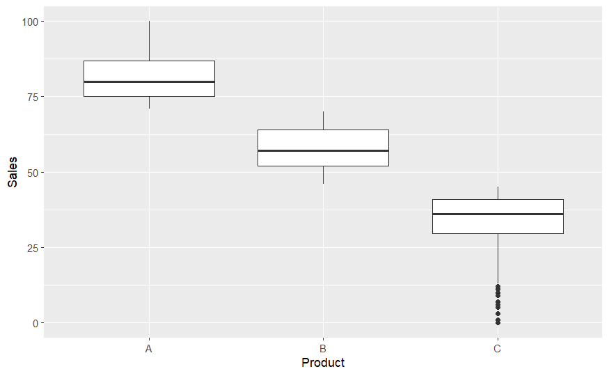
ggplot(BR_data) +
aes(x = Product, y = Sales) +
geom_boxplot()
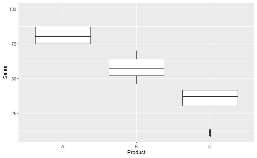
# dealing with outliers
Q <- quantile(BR_data$Sales, probs=c(.25, .75), na.rm = FALSE) #find the 25th and the 75th percentile
iqr <- IQR(BR_data$Sales) #Interquartile range
up <-  Q[2]+1.5*iqr # Upper Range
low<- Q[1]-1.5*iqr # Lower Range

BR_data_eliminated<- subset(BR_data, BR_data$Sales > (Q[1] - 1.5*iqr) & BR_data$Sales < (Q[2]+1.5*iqr))

ggplot(BR_data_eliminated) +
  aes(x = Product, y = Sales) +
  geom_boxplot()
# 4th evaluation and post-hoc
aov_BR_wO <- aov(Sales ~ Product, data = BR_data_eliminated)
summary(aov_BR_wO) # high significant influence of Factor Product on DV Sales
##              Df Sum Sq Mean Sq F value Pr(>F)
## Product       2 247899  123950    2273 <2e-16 ***
## Residuals   989  53941      55
## ---
## Signif. codes:  0 '***' 0.001 '**' 0.01 '*' 0.05 '.' 0.1 ' ' 1
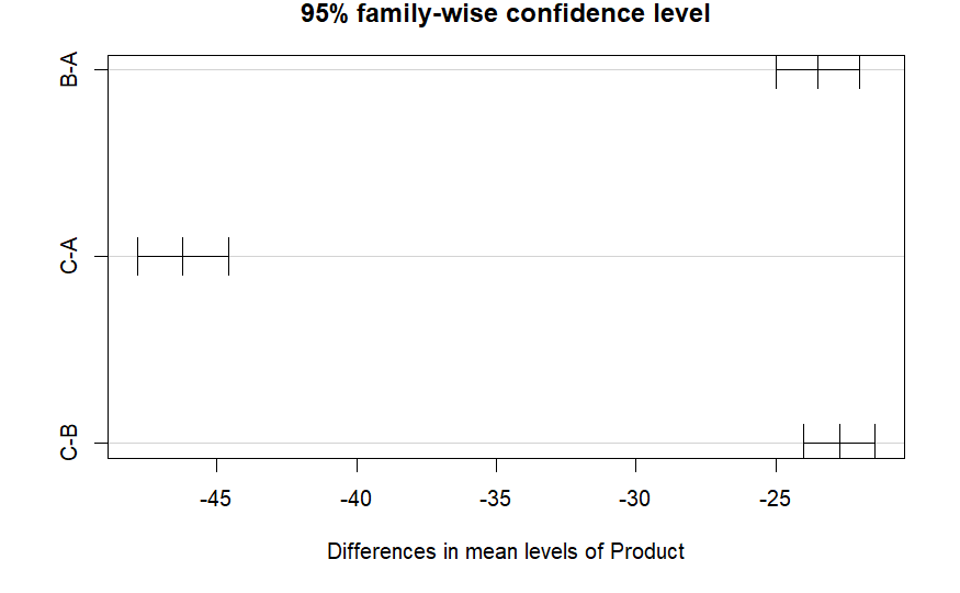
# post-hoc
TukeyHSD(aov_BR_wO) # all products are significantly different in terms of sales
##   Tukey multiple comparisons of means
##     95% family-wise confidence level
##
## Fit: aov(formula = Sales ~ Product, data = BR_data_eliminated)
##
## $Product
##          diff       lwr       upr p adj
## B-A -23.50199 -24.98491 -22.01908     0
## C-A -46.22270 -47.85003 -44.59538     0
## C-B -22.72071 -23.99197 -21.44945     0
plot(TukeyHSD(aov_BR_wO))
ANCOVA
# We assume that the TV_spent variable has a prospective influence and therefore is a covariate
# Note. TV_spent goes first with no interaction to control for its effect
acov_BR_wO <- aov(Sales ~ TV_spent + Product, data = BR_data_eliminated)
summary(acov_BR_wO)
##              Df Sum Sq Mean Sq F value Pr(>F)
## TV_spent      1 227481  227481  6491.0 <2e-16 ***
## Product       2  39734   19867   566.9 <2e-16 ***
## Residuals   988  34625      35
## ---
## Signif. codes:  0 '***' 0.001 '**' 0.01 '*' 0.05 '.' 0.1 ' ' 1
# post-hoc shows that there are still sign. effect from product on sales after controlling for TV_spent
acov_BR_PH <- BR_data_eliminated %>%
  emmeans_test(
    Sales ~ Product, covariate = TV_spent,
    p.adjust.method = "bonferroni"
  )
acov_BR_PH
## # A tibble: 3 x 9
##   term             .y.   group1 group2    df stati~1         p     p.adj p.adj~2
## * <chr>            <chr> <chr>  <chr>  <dbl>   <dbl>     <dbl>     <dbl> <chr>
## 1 TV_spent*Product Sales A      B        988    25.2 6.74e-109 2.02e-108 ****
## 2 TV_spent*Product Sales A      C        988    33.6 7.83e-166 2.35e-165 ****
## 3 TV_spent*Product Sales B      C        988    25.9 2.55e-113 7.65e-113 ****
## # ... with abbreviated variable names 1: statistic, 2: p.adj.signif
# see the estimated marginal means
get_emmeans(acov_BR_PH)
## # A tibble: 3 x 8
##   TV_spent Product emmean    se    df conf.low conf.high method
##      <dbl> <fct>    <dbl> <dbl> <dbl>    <dbl>     <dbl> <chr>
## 1     50.2 A         72.2 0.578   988     71.0      73.3 Emmeans test
## 2     50.2 B         56.7 0.264   988     56.2      57.3 Emmeans test
## 3     50.2 C         42.3 0.467   988     41.4      43.2 Emmeans test
t-test
# divide data set in low (<=50) and high (>=51) trust
BR_data_eliminated <- BR_data_eliminated %>%
  mutate(Trust_binary = case_when(
    Brand_trust<=50 ~ "low",
    Brand_trust>=51 ~ "high"))

# first some descriptives
BR_data_eliminated %>%
  group_by(Trust_binary) %>%
  summarise_at(vars(Sales), list(Sales_mean = mean))
## # A tibble: 2 x 2
##   Trust_binary Sales_mean
##   <chr>             <dbl>
## 1 high               60.4
## 2 low                50.6
# is this difference random or systematical?
t.test(Sales ~ Trust_binary, data = BR_data_eliminated) # the binary level of trust seems to have an sign influence on sales
##
##  Welch Two Sample t-test
##
## data:  Sales by Trust_binary
## t = 9.241, df = 988, p-value < 2.2e-16
## alternative hypothesis: true difference in means between group high and group low is not equal to 0
## 95 percent confidence interval:
##   7.744993 11.921207
## sample estimates:
## mean in group high  mean in group low
##           60.42562           50.59252
Correlation and linear Regression
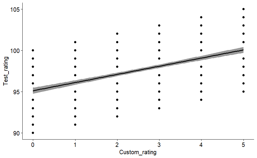
ggscatter(BR_data_eliminated, x = "Custom_rating", y = "Test_rating",
          add = "reg.line", conf.int = TRUE) # visual inspection indicates medium correlation
## `geom_smooth()` using formula = 'y ~ x'
# next check for normality assumption on both variables using our old friend Shapiro
shapiro.test(BR_data_eliminated$Custom_rating) # p <0.05, normality assumption violated
##
##  Shapiro-Wilk normality test
##
## data:  BR_data_eliminated$Custom_rating
## W = 0.90503, p-value < 2.2e-16
shapiro.test(BR_data_eliminated$Test_rating) # p <0.05, normality assumption violated
##
##  Shapiro-Wilk normality test
##
## data:  BR_data_eliminated$Test_rating
## W = 0.97448, p-value = 3.433e-12
# now correlation check
# if shapiro test are not significant use 'method = pearson'. Other you can use 'spearman' or 'kendall'
cor.test(BR_data_eliminated$Custom_rating, BR_data_eliminated$Test_rating, method = "pearson")
##
##  Pearson's product-moment correlation
##
## data:  BR_data_eliminated$Custom_rating and BR_data_eliminated$Test_rating
## t = 16.233, df = 990, p-value < 2.2e-16
## alternative hypothesis: true correlation is not equal to 0
## 95 percent confidence interval:
##  0.4078978 0.5062937
## sample estimates:
##       cor
## 0.4584998
cor.test(BR_data_eliminated$Custom_rating, BR_data_eliminated$Test_rating, method = "spearman")
## Warning in cor.test.default(BR_data_eliminated$Custom_rating,
## BR_data_eliminated$Test_rating, : Cannot compute exact p-value with ties

##
##  Spearman's rank correlation rho
##
## data:  BR_data_eliminated$Custom_rating and BR_data_eliminated$Test_rating
## S = 91159249, p-value < 2.2e-16
## alternative hypothesis: true rho is not equal to 0
## sample estimates:
##       rho
## 0.4397041
cor.test(BR_data_eliminated$Custom_rating, BR_data_eliminated$Test_rating, method = "kendall")
##
##  Kendall's rank correlation tau
##
## data:  BR_data_eliminated$Custom_rating and BR_data_eliminated$Test_rating
## z = 14.448, p-value < 2.2e-16
## alternative hypothesis: true tau is not equal to 0
## sample estimates:
##       tau
## 0.3424049
# compute correlation matrix
# preselect numeric columns
BR_Cor_data <- BR_data_eliminated[, c(1,2,3,4,5,6,7,8,9)]
#compute correlation matrix
M_cor_BR <- cor(BR_Cor_data)
# do some rounding to 2 decimal places
round(M_cor_BR, 2)
##                TV_spent SoMed_spent Custom_rating Test_rating Dura_score
## TV_spent           1.00        0.63          0.04        0.01      -0.04
## SoMed_spent        0.63        1.00          0.03       -0.01      -0.05
## Custom_rating      0.04        0.03          1.00        0.46      -0.05
## Test_rating        0.01       -0.01          0.46        1.00       0.02
## Dura_score        -0.04       -0.05         -0.05        0.02       1.00
## Function_score    -0.04       -0.07         -0.05        0.01       0.82
## Sales              0.87        0.52          0.17        0.07       0.15
## Brand_trust        0.30        0.46          0.03        0.13       0.68
## Emotion_appeal    -0.04       -0.07          0.02        0.05       0.79
##                Function_score Sales Brand_trust Emotion_appeal
## TV_spent                -0.04  0.87        0.30          -0.04
## SoMed_spent             -0.07  0.52        0.46          -0.07
## Custom_rating           -0.05  0.17        0.03           0.02
## Test_rating              0.01  0.07        0.13           0.05
## Dura_score               0.82  0.15        0.68           0.79
## Function_score           1.00  0.11        0.83           0.98
## Sales                    0.11  1.00        0.38           0.13
## Brand_trust              0.83  0.38        1.00           0.81
## Emotion_appeal           0.98  0.13        0.81           1.00
# if you want to do it in one step (viz&compute)
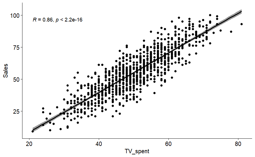
ggscatter(BR_data_eliminated, x = "TV_spent", y = "Sales",
add = "reg.line", conf.int = TRUE,
cor.coef = TRUE, cor.method = "spearman")
## `geom_smooth()` using formula = 'y ~ x'
# Simple Regression
SR_BR_data <- lm(Sales ~ TV_spent, data = BR_data_eliminated)
summary(SR_BR_data)
##
## Call:
## lm(formula = Sales ~ TV_spent, data = BR_data_eliminated)
##
## Residuals:
##      Min       1Q   Median       3Q      Max
## -25.8880  -5.6201  -0.2541   5.7770  24.6689
##
## Coefficients:
##             Estimate Std. Error t value Pr(>|t|)
## (Intercept) -22.2467     1.4373  -15.48   <2e-16 ***
## TV_spent      1.5464     0.0281   55.03   <2e-16 ***
## ---
## Signif. codes:  0 '***' 0.001 '**' 0.01 '*' 0.05 '.' 0.1 ' ' 1
##
## Residual standard error: 8.667 on 990 degrees of freedom
## Multiple R-squared:  0.7536, Adjusted R-squared:  0.7534
## F-statistic:  3029 on 1 and 990 DF,  p-value: < 2.2e-16
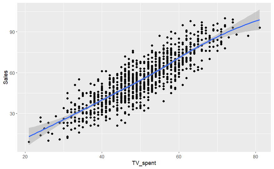
# plot the regression in nice
ggplot(BR_data_eliminated, aes(x = TV_spent, y = Sales)) +
  geom_point() +
  stat_smooth()
# Multiple Regression
MR_BR_data <- lm(Sales ~ TV_spent + Brand_trust, data = BR_data_eliminated)
summary(MR_BR_data) # see estimates and only slightly increased R-squared
##
## Call:
## lm(formula = Sales ~ TV_spent + Brand_trust, data = BR_data_eliminated)
##
## Residuals:
##      Min       1Q   Median       3Q      Max
## -25.9497  -5.6527  -0.1759   6.0495  23.7861
##
## Coefficients:
##              Estimate Std. Error t value Pr(>|t|)
## (Intercept) -25.63806    1.43917 -17.815   <2e-16 ***
## TV_spent      1.47318    0.02836  51.945   <2e-16 ***
## Brand_trust   0.14123    0.01619   8.726   <2e-16 ***
## ---
## Signif. codes:  0 '***' 0.001 '**' 0.01 '*' 0.05 '.' 0.1 ' ' 1
##
## Residual standard error: 8.355 on 989 degrees of freedom
## Multiple R-squared:  0.7713, Adjusted R-squared:  0.7708
## F-statistic:  1667 on 2 and 989 DF,  p-value: < 2.2e-16
# compute standardized coefficients
lm.beta(MR_BR_data) # TV_spent nearly 4 times the influence on Sales
##    TV_spent Brand_trust
##   0.8270212   0.1389241
EFA, CFA and Scale Evaluation
BR_FA_data <- BR_data_eliminated[, c(2,3,4,5,6,7)] # note that these data is not the best fitting data for factor analysis cause these are scores and no items

# is sample adequate using KMO criterion
psych::KMO(BR_FA_data) # rule of thumb KMO > 0.5
## Kaiser-Meyer-Olkin factor adequacy
## Call: psych::KMO(r = BR_FA_data)
## Overall MSA =  0.5
## MSA for each item =
##    SoMed_spent  Custom_rating    Test_rating     Dura_score Function_score
##           0.48           0.50           0.51           0.51           0.51
##          Sales
##           0.50
# check for significancy of the multiple correlations using Bartlett-test
psych::cortest.bartlett(BR_FA_data) # is significant
## R was not square, finding R from data

## $chisq
## [1] 1726.557
##
## $p.value
## [1] 0
##
## $df
## [1] 15
# now we can start our factor analyses
# Starting with an explorative factor analysis (EFA)
# Parallel analysis
psych::fa.parallel(BR_FA_data)
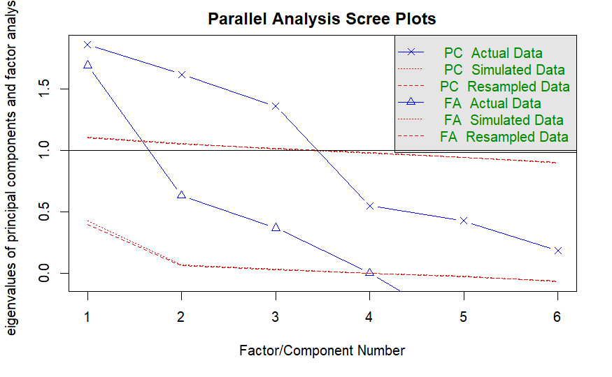
## Parallel analysis suggests that the number of factors = 3 and the number of components = 3
BR_EFA <- fa(BR_FA_data, nfactors = 3)
BR_EFA # 3 factor solution and 67% variance explained
## Factor Analysis using method =  minres
## Call: fa(r = BR_FA_data, nfactors = 3)
## Standardized loadings (pattern matrix) based upon correlation matrix
##                  MR1   MR2   MR3   h2     u2 com
## SoMed_spent    -0.06 -0.04  0.86 0.75 0.2533 1.0
## Custom_rating  -0.01  1.00  0.00 1.00 0.0049 1.0
## Test_rating     0.04  0.46 -0.02 0.21 0.7863 1.0
## Dura_score      0.97 -0.01  0.01 0.94 0.0579 1.0
## Function_score  0.84 -0.01 -0.02 0.71 0.2900 1.0
## Sales           0.16  0.12  0.61 0.42 0.5770 1.2
##
##                        MR1  MR2  MR3
## SS loadings           1.68 1.23 1.12
## Proportion Var        0.28 0.20 0.19
## Cumulative Var        0.28 0.48 0.67
## Proportion Explained  0.42 0.30 0.28
## Cumulative Proportion 0.42 0.72 1.00
##
##  With factor correlations of
##       MR1   MR2  MR3
## MR1  1.00 -0.04 0.00
## MR2 -0.04  1.00 0.08
## MR3  0.00  0.08 1.00
##
## Mean item complexity =  1
## Test of the hypothesis that 3 factors are sufficient.
##
## The degrees of freedom for the null model are  15  and the objective function was  1.75 with Chi Square of  1726.56
## The degrees of freedom for the model are 0  and the objective function was  0
##
## The root mean square of the residuals (RMSR) is  0
## The df corrected root mean square of the residuals is  NA
##
## The harmonic number of observations is  992 with the empirical chi square  0.03  with prob <  NA
## The total number of observations was  992  with Likelihood Chi Square =  0.13  with prob <  NA
##
## Tucker Lewis Index of factoring reliability =  -Inf
## Fit based upon off diagonal values = 1
## Measures of factor score adequacy
##                                                    MR1  MR2  MR3
## Correlation of (regression) scores with factors   0.97 1.00 0.88
## Multiple R square of scores with factors          0.95 1.00 0.78
## Minimum correlation of possible factor scores     0.90 0.99 0.57
# Next Confirmatory factor analysis (CFA)
# To demonstrate CFA we do need a different data set
# We use an inbuilt data set which you can load as follows:
CFA_HS_data <- lavaan::HolzingerSwineford1939 # data set on pupils and their abilities
CFA_syntx <- '
  visual =~ x1 + x2 + x3
  textual =~ x4 + x5 + x6
  speed =~ x7 + x8 + x9
  '# define CFA model

# fit the model
BR_CFA <- lavaan::cfa(CFA_syntx, data = CFA_HS_data)

# check summary
summary(BR_CFA, fit.measures = T)
## lavaan 0.6.13 ended normally after 35 iterations
##
##   Estimator                                         ML
##   Optimization method                           NLMINB
##   Number of model parameters                        21
##
##   Number of observations                           301
##
## Model Test User Model:
##
##   Test statistic                                85.306
##   Degrees of freedom                                24
##   P-value (Chi-square)                           0.000
##
## Model Test Baseline Model:
##
##   Test statistic                               918.852
##   Degrees of freedom                                36
##   P-value                                        0.000
##
## User Model versus Baseline Model:
##
##   Comparative Fit Index (CFI)                    0.931
##   Tucker-Lewis Index (TLI)                       0.896
##
## Loglikelihood and Information Criteria:
##
##   Loglikelihood user model (H0)              -3737.745
##   Loglikelihood unrestricted model (H1)      -3695.092
##
##   Akaike (AIC)                                7517.490
##   Bayesian (BIC)                              7595.339
##   Sample-size adjusted Bayesian (SABIC)       7528.739
##
## Root Mean Square Error of Approximation:
##
##   RMSEA                                          0.092
##   90 Percent confidence interval - lower         0.071
##   90 Percent confidence interval - upper         0.114
##   P-value H_0: RMSEA <= 0.050                    0.001
##   P-value H_0: RMSEA >= 0.080                    0.840
##
## Standardized Root Mean Square Residual:
##
##   SRMR                                           0.065
##
## Parameter Estimates:
##
##   Standard errors                             Standard
##   Information                                 Expected
##   Information saturated (h1) model          Structured
##
## Latent Variables:
##                    Estimate  Std.Err  z-value  P(>|z|)
##   visual =~
##     x1                1.000
##     x2                0.554    0.100    5.554    0.000
##     x3                0.729    0.109    6.685    0.000
##   textual =~
##     x4                1.000
##     x5                1.113    0.065   17.014    0.000
##     x6                0.926    0.055   16.703    0.000
##   speed =~
##     x7                1.000
##     x8                1.180    0.165    7.152    0.000
##     x9                1.082    0.151    7.155    0.000
##
## Covariances:
##                    Estimate  Std.Err  z-value  P(>|z|)
##   visual ~~
##     textual           0.408    0.074    5.552    0.000
##     speed             0.262    0.056    4.660    0.000
##   textual ~~
##     speed             0.173    0.049    3.518    0.000
##
## Variances:
##                    Estimate  Std.Err  z-value  P(>|z|)
##    .x1                0.549    0.114    4.833    0.000
##    .x2                1.134    0.102   11.146    0.000
##    .x3                0.844    0.091    9.317    0.000
##    .x4                0.371    0.048    7.779    0.000
##    .x5                0.446    0.058    7.642    0.000
##    .x6                0.356    0.043    8.277    0.000
##    .x7                0.799    0.081    9.823    0.000
##    .x8                0.488    0.074    6.573    0.000
##    .x9                0.566    0.071    8.003    0.000
##     visual            0.809    0.145    5.564    0.000
##     textual           0.979    0.112    8.737    0.000
##     speed             0.384    0.086    4.451    0.000
# check how to 'statistically' improve the model - please dont do this blindly but consider if it is also reasonable
modindices(BR_CFA, sort = TRUE, maximum.number = 5)
##        lhs op rhs     mi    epc sepc.lv sepc.all sepc.nox
## 30  visual =~  x9 36.411  0.577   0.519    0.515    0.515
## 76      x7 ~~  x8 34.145  0.536   0.536    0.859    0.859
## 28  visual =~  x7 18.631 -0.422  -0.380   -0.349   -0.349
## 78      x8 ~~  x9 14.946 -0.423  -0.423   -0.805   -0.805
## 33 textual =~  x3  9.151 -0.272  -0.269   -0.238   -0.238
# plot the CFA model with 'std' estimates
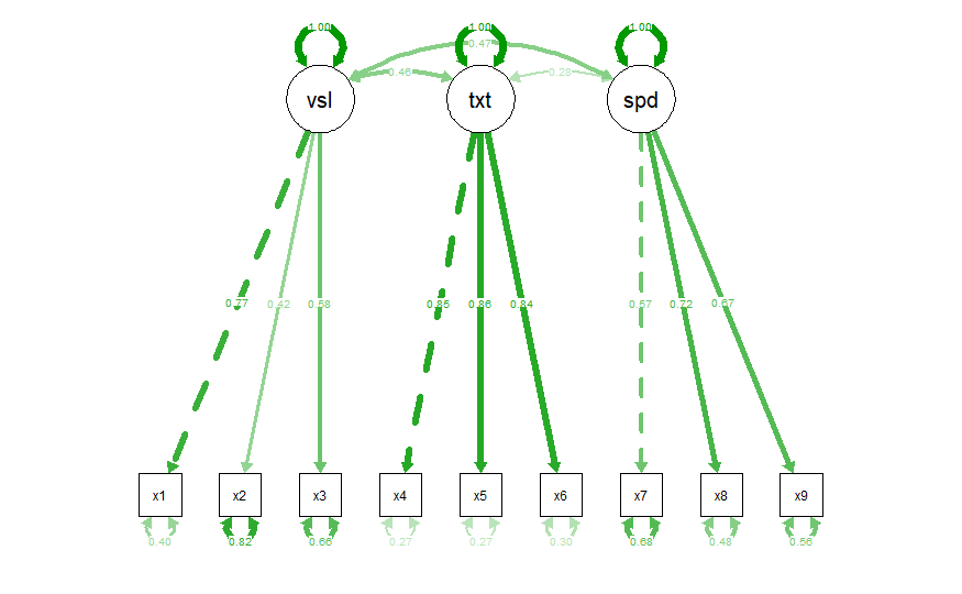
semPlot::semPaths(BR_CFA, "std")
# Addtition: Scale evaluation
# Alpha
alpha(subset(CFA_HS_data, select = c(x4, x5, x6))) # rule of thumb > 0.6
## Number of categories should be increased  in order to count frequencies.

##
## Reliability analysis
## Call: alpha(x = subset(CFA_HS_data, select = c(x4, x5, x6)))
##
##   raw_alpha std.alpha G6(smc) average_r S/N   ase mean  sd median_r
##       0.88      0.88    0.84      0.72 7.7 0.011  3.2 1.1     0.72
##
##     95% confidence boundaries
##          lower alpha upper
## Feldt     0.86  0.88  0.90
## Duhachek  0.86  0.88  0.91
##
##  Reliability if an item is dropped:
##    raw_alpha std.alpha G6(smc) average_r S/N alpha se var.r med.r
## x4      0.83      0.84    0.72      0.72 5.1    0.019    NA  0.72
## x5      0.83      0.83    0.70      0.70 4.8    0.020    NA  0.70
## x6      0.84      0.85    0.73      0.73 5.5    0.018    NA  0.73
##
##  Item statistics
##      n raw.r std.r r.cor r.drop mean  sd
## x4 301  0.90  0.90  0.82   0.78  3.1 1.2
## x5 301  0.92  0.91  0.84   0.79  4.3 1.3
## x6 301  0.89  0.90  0.81   0.77  2.2 1.1
# CR - Composite Reliability
# only for specific factor
compRelSEM(BR_CFA, omit.factors = c("speed", "visual"), return.total = TRUE) # rule of thumb > 0.7
## textual
##   0.885
# for all indicators
compRelSEM(BR_CFA, return.total = TRUE)
##  visual textual   speed   total
##   0.612   0.885   0.686   0.860
# AVE - Average Variance Extracted
AVE(BR_CFA) # rule of thumb > 0.5
##  visual textual   speed
##   0.371   0.721   0.424
SEM in Lavaan
# latent variable analysis
# '=~' latent definition
# '~' regression path
# '~~' covaraince/correlation
# we switch back to our initial data set from the rest of the script
# before analyzing SEM you need to build a model which is similar to CFA except you also build regression paths
BR_SEM <- '
  # measurement model
    Ad_spent =~ TV_spent + SoMed_spent
    O_review =~ Custom_rating + Test_rating
    Prod_qual =~ Dura_score + Function_score
    Brand_repu =~ Sales + Brand_trust + Emotion_appeal
  # regressions
    Brand_repu ~ Ad_spent + O_review + Prod_qual
'

BR_SEM_fit <- sem(BR_SEM, data = BR_data_eliminated) # warning messages indicates Heywood case (interpret with caution; maybe varaible are very strong correlated?)
summary(BR_SEM_fit, standardized = TRUE, fit.measures = T)
## lavaan 0.6.13 ended normally after 239 iterations
##
##   Estimator                                         ML
##   Optimization method                           NLMINB
##   Number of model parameters                        24
##
##   Number of observations                           992
##
## Model Test User Model:
##
##   Test statistic                              3227.393
##   Degrees of freedom                                21
##   P-value (Chi-square)                           0.000
##
## Model Test Baseline Model:
##
##   Test statistic                             10112.833
##   Degrees of freedom                                36
##   P-value                                        0.000
##
## User Model versus Baseline Model:
##
##   Comparative Fit Index (CFI)                    0.682
##   Tucker-Lewis Index (TLI)                       0.455
##
## Loglikelihood and Information Criteria:
##
##   Loglikelihood user model (H0)             -28715.834
##   Loglikelihood unrestricted model (H1)     -27102.138
##
##   Akaike (AIC)                               57479.668
##   Bayesian (BIC)                             57597.262
##   Sample-size adjusted Bayesian (SABIC)      57521.037
##
## Root Mean Square Error of Approximation:
##
##   RMSEA                                          0.392
##   90 Percent confidence interval - lower         0.381
##   90 Percent confidence interval - upper         0.404
##   P-value H_0: RMSEA <= 0.050                    0.000
##   P-value H_0: RMSEA >= 0.080                    1.000
##
## Standardized Root Mean Square Residual:
##
##   SRMR                                           0.162
##
## Parameter Estimates:
##
##   Standard errors                             Standard
##   Information                                 Expected
##   Information saturated (h1) model          Structured
##
## Latent Variables:
##                    Estimate  Std.Err  z-value  P(>|z|)   Std.lv  Std.all
##   Ad_spent =~
##     TV_spent          1.000                               6.471    0.661
##     SoMed_spent       2.195    0.085   25.886    0.000   14.208    0.954
##   O_review =~
##     Custom_rating     1.000                               1.002    0.584
##     Test_rating       2.896    0.207   14.015    0.000    2.901    0.785
##   Prod_qual =~
##     Dura_score        1.000                               2.034    0.819
##     Function_score   11.844    0.267   44.349    0.000   24.090    0.998
##   Brand_repu =~
##     Sales             1.000                               5.324    0.305
##     Brand_trust       2.974    0.256   11.627    0.000   15.831    0.923
##     Emotion_appeal    3.408    0.294   11.579    0.000   18.141    0.882
##
## Regressions:
##                    Estimate  Std.Err  z-value  P(>|z|)   Std.lv  Std.all
##   Brand_repu ~
##     Ad_spent          0.315    0.029   10.732    0.000    0.383    0.383
##     O_review          0.691    0.076    9.120    0.000    0.130    0.130
##     Prod_qual         2.616    0.229   11.411    0.000    1.000    1.000
##
## Covariances:
##                    Estimate  Std.Err  z-value  P(>|z|)   Std.lv  Std.all
##   Ad_spent ~~
##     O_review          0.043    0.261    0.167    0.868    0.007    0.007
##     Prod_qual        -0.935    0.440   -2.125    0.034   -0.071   -0.071
##   O_review ~~
##     Prod_qual        -0.021    0.079   -0.268    0.789   -0.010   -0.010
##
## Variances:
##                    Estimate  Std.Err  z-value  P(>|z|)   Std.lv  Std.all
##    .TV_spent         54.015    2.504   21.572    0.000   54.015    0.563
##    .SoMed_spent      19.846    3.129    6.342    0.000   19.846    0.090
##    .Custom_rating     1.936    0.106   18.206    0.000    1.936    0.659
##    .Test_rating       5.245    0.565    9.278    0.000    5.245    0.384
##    .Dura_score        2.034    0.092   22.023    0.000    2.034    0.330
##    .Function_score    2.030    1.932    1.051    0.293    2.030    0.003
##    .Sales           275.933   12.064   22.873    0.000  275.933    0.907
##    .Brand_trust      43.793    2.097   20.888    0.000   43.793    0.149
##    .Emotion_appeal   94.113    4.265   22.068    0.000   94.113    0.222
##     Ad_spent         41.878    3.612   11.595    0.000    1.000    1.000
##     O_review          1.003    0.117    8.597    0.000    1.000    1.000
##     Prod_qual         4.137    0.262   15.793    0.000    1.000    1.000
##    .Brand_repu       -3.015    0.522   -5.779    0.000   -0.106   -0.106
# modification indices (bad example)
modindices(BR_SEM_fit, sort = TRUE, maximum.number = 10)
##               lhs op            rhs      mi     epc sepc.lv sepc.all sepc.nox
## 35       Ad_spent =~ Emotion_appeal 858.570  -1.919 -12.416   -0.604   -0.604
## 49      Prod_qual =~ Emotion_appeal 762.683  14.253  28.990    1.409    1.409
## 34       Ad_spent =~    Brand_trust 652.973   1.453   9.402    0.548    0.548
## 48      Prod_qual =~    Brand_trust 585.142 -10.920 -22.211   -1.294   -1.294
## 61       TV_spent ~~          Sales 507.951  89.912  89.912    0.736    0.736
## 69    SoMed_spent ~~    Brand_trust 397.665  79.602  79.602    2.700    2.700
## 70    SoMed_spent ~~ Emotion_appeal 359.442 -86.370 -86.370   -1.999   -1.999
## 33       Ad_spent =~          Sales 256.114   1.359   8.797    0.504    0.504
## 47      Prod_qual =~          Sales 111.753  -4.858  -9.882   -0.567   -0.567
## 88 Function_score ~~ Emotion_appeal  85.396  53.391  53.391    3.863    3.863
# second better working example
SEM_PD_data <- lavaan::PoliticalDemocracy
?PoliticalDemocracy# examine how the industrialization 1960 of a country and the democracy 1960 influence the democratic degree in 1965
# build the model #1
SEM_PD <- '
  # measurement model
    industr60 =~ x1 + x2 + x3
    democra60 =~ y1 + y2 + y3 + y4
    democra65 =~ y5 + y6 + y7 + y8
  # regressions
    democra60 ~ industr60
    democra65 ~ industr60 + democra60
'
# fit the model and look at summary (a guide to evaluate SEM models is attached to the added materials)
fit_PD <- sem(SEM_PD, data = PoliticalDemocracy)
summary(fit_PD, standardized = TRUE, fit.measures = T)
## lavaan 0.6.13 ended normally after 42 iterations
##
##   Estimator                                         ML
##   Optimization method                           NLMINB
##   Number of model parameters                        25
##
##   Number of observations                            75
##
## Model Test User Model:
##
##   Test statistic                                72.462
##   Degrees of freedom                                41
##   P-value (Chi-square)                           0.002
##
## Model Test Baseline Model:
##
##   Test statistic                               730.654
##   Degrees of freedom                                55
##   P-value                                        0.000
##
## User Model versus Baseline Model:
##
##   Comparative Fit Index (CFI)                    0.953
##   Tucker-Lewis Index (TLI)                       0.938
##
## Loglikelihood and Information Criteria:
##
##   Loglikelihood user model (H0)              -1564.959
##   Loglikelihood unrestricted model (H1)      -1528.728
##
##   Akaike (AIC)                                3179.918
##   Bayesian (BIC)                              3237.855
##   Sample-size adjusted Bayesian (SABIC)       3159.062
##
## Root Mean Square Error of Approximation:
##
##   RMSEA                                          0.101
##   90 Percent confidence interval - lower         0.061
##   90 Percent confidence interval - upper         0.139
##   P-value H_0: RMSEA <= 0.050                    0.021
##   P-value H_0: RMSEA >= 0.080                    0.827
##
## Standardized Root Mean Square Residual:
##
##   SRMR                                           0.055
##
## Parameter Estimates:
##
##   Standard errors                             Standard
##   Information                                 Expected
##   Information saturated (h1) model          Structured
##
## Latent Variables:
##                    Estimate  Std.Err  z-value  P(>|z|)   Std.lv  Std.all
##   industr60 =~
##     x1                1.000                               0.669    0.920
##     x2                2.182    0.139   15.714    0.000    1.461    0.973
##     x3                1.819    0.152   11.956    0.000    1.218    0.872
##   democra60 =~
##     y1                1.000                               2.201    0.845
##     y2                1.354    0.175    7.755    0.000    2.980    0.760
##     y3                1.044    0.150    6.961    0.000    2.298    0.705
##     y4                1.300    0.138    9.412    0.000    2.860    0.860
##   democra65 =~
##     y5                1.000                               2.084    0.803
##     y6                1.258    0.164    7.651    0.000    2.623    0.783
##     y7                1.282    0.158    8.137    0.000    2.673    0.819
##     y8                1.310    0.154    8.529    0.000    2.730    0.847
##
## Regressions:
##                    Estimate  Std.Err  z-value  P(>|z|)   Std.lv  Std.all
##   democra60 ~
##     industr60         1.474    0.392    3.763    0.000    0.448    0.448
##   democra65 ~
##     industr60         0.453    0.220    2.064    0.039    0.146    0.146
##     democra60         0.864    0.113    7.671    0.000    0.913    0.913
##
## Variances:
##                    Estimate  Std.Err  z-value  P(>|z|)   Std.lv  Std.all
##    .x1                0.082    0.020    4.180    0.000    0.082    0.154
##    .x2                0.118    0.070    1.689    0.091    0.118    0.053
##    .x3                0.467    0.090    5.174    0.000    0.467    0.240
##    .y1                1.942    0.395    4.910    0.000    1.942    0.286
##    .y2                6.490    1.185    5.479    0.000    6.490    0.422
##    .y3                5.340    0.943    5.662    0.000    5.340    0.503
##    .y4                2.887    0.610    4.731    0.000    2.887    0.261
##    .y5                2.390    0.447    5.351    0.000    2.390    0.355
##    .y6                4.343    0.796    5.456    0.000    4.343    0.387
##    .y7                3.510    0.668    5.252    0.000    3.510    0.329
##    .y8                2.940    0.586    5.019    0.000    2.940    0.283
##     industr60         0.448    0.087    5.169    0.000    1.000    1.000
##    .democra60         3.872    0.893    4.338    0.000    0.799    0.799
##    .democra65         0.115    0.200    0.575    0.565    0.026    0.026
# compute mod indices
modindices(fit_PD, sort = TRUE, maximum.number = 10)
##           lhs op rhs    mi    epc sepc.lv sepc.all sepc.nox
## 88         y2 ~~  y6 9.279  2.129   2.129    0.401    0.401
## 104        y6 ~~  y8 8.668  1.513   1.513    0.423    0.423
## 81         y1 ~~  y5 8.183  0.884   0.884    0.410    0.410
## 93         y3 ~~  y6 6.574 -1.590  -1.590   -0.330   -0.330
## 79         y1 ~~  y3 5.204  1.024   1.024    0.318    0.318
## 86         y2 ~~  y4 4.911  1.432   1.432    0.331    0.331
## 94         y3 ~~  y7 4.088  1.152   1.152    0.266    0.266
## 33  industr60 =~  y5 4.007  0.762   0.510    0.197    0.197
## 54         x1 ~~  y2 3.785 -0.192  -0.192   -0.263   -0.263
## 32  industr60 =~  y4 3.568  0.811   0.543    0.163    0.163
Fit indices (CFI, TLI, SRMR, test statistic/df) for this model are already quite ok. Only RMSEA is not < 0.08. Regression coefficients show that there is a singificant effect from the degree of industrialization in the 60s on the degree of democracy in 65. And the degree of democracy in the 60s works as a partial mediator. Based on the modification indices we could statistically improve outr model by correlating e.g. y6 and y8 (y6 ~~ y8). You are welcome to try it out for yourself!
Hope you had fun with this script :) Cheers, Maik